4 Differential Drive
4.1 Dynamics
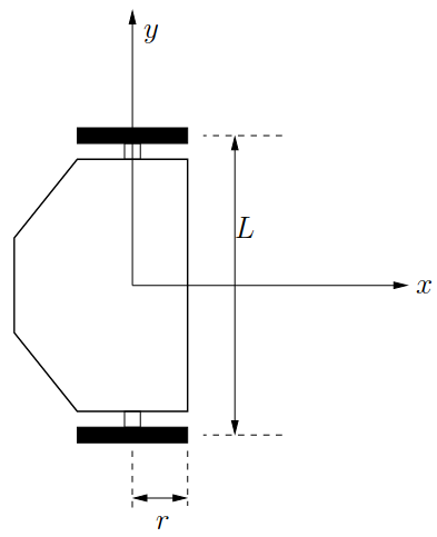
- Parameters
- \(r\): radius of the wheels [m]
- \(L\): distance between the wheels [m]
- State: \(\mathbf{x}= \begin{pmatrix}x, y, \theta\end{pmatrix}^\top\) [m, m, rad] (position and orientation of the robot in the world frame)
- Action: \(\mathbf{u}= \begin{pmatrix} u_l, u_r \end{pmatrix}^\top\) [rad/s, rad/s] (angular velocity of the left and right wheels, respectively)
- Dynamics: \[ \begin{aligned} \dot x &= \frac{r}{2} (u_l + u_r) \cos \theta \\ \dot y &= \frac{r}{2} (u_l + u_r) \sin \theta \\ \dot \theta &= \frac{r}{L} (u_r - u_l) \end{aligned} \]
4.1.1 Relationship to Unicycle
There is a linear relationship between the differential drive and the unicycle. One can substitute actions to \(v = \frac{r}{2} (u_l + u_r)\) and \(\omega = \frac{r}{L} (u_r - u_l)\) to get \[ \begin{aligned} \dot x &= v \cos \theta \\ \dot y &= v \sin \theta \\ \dot \theta &= \omega \end{aligned} \]
Then, the “original” actions can be computed as \[\begin{aligned} u_l &= \frac{2v-L\omega}{2r}\\ u_r &= \frac{2v + L\omega}{2r} \end{aligned} \]
\[ 2v = r (u_l + u_r) \tag{4.1}\]
\[ L\omega = r (u_r - u_l) \tag{4.2}\]
Adding Equation 4.1 and Equation 4.2:
\[ \begin{aligned} 2v + L\omega = r (u_l + u_r + u_r - u_l) = 2 r u_r\\ u_r = \frac{2v + L\omega}{2 r} \end{aligned} \tag{4.3}\]
Substituting Equation 4.3 in Equation 4.1: \[ \begin{aligned} 2v = r (u_l + u_r) = r (u_l + \frac{2v + L\omega}{2 r}) = r u_l + v + \frac{L\omega}{2}\\ u_l = \frac{2v - v - \frac{L\omega}{2}}{r} = \frac{2v - L \omega}{2 r} \end{aligned} \tag{4.4}\]
4.2 Differential Flatness
Pick flat outputs \(\mathbf{z}(t) = (x(t), y(t))^\top\), i.e., the position of the robot. Then we can compute all necessary variables if \(\mathbf{z}(t)\) is at least C2-continuous. \[ \begin{aligned} \mathbf{x}(t) &= g_x(\mathbf{z}, \dot{\mathbf{z}}) = \left(x, y, \arctan \left(\frac{\dot y}{\dot x}\right)\right)\\ \mathbf{u}(t) &= g_u(\dot{\mathbf{z}}, \ddot{\mathbf{z}}) = \left(\frac{2v-L\omega}{2r}, \frac{2v + L\omega}{2r}\right), \text{ where }\\ v &= {\color{red} \pm}\sqrt{\dot y^2 + \dot x^2}\\ \omega &= \frac{\dot x \ddot y - \dot y \ddot x}{\dot x^2 + \dot y^2} \end{aligned} \]
One can apply the same differential flatness result from the unicycle, followed by the linear mapping derived earlier to recover the actual actions \(g_u\).
4.3 Invariance
The dynamics are translation-invariant.
4.4 Controllers
4.4.1 Geometric Controller
This is the same controller as for the unicycle proposed in (Kanayama et al. (1990)), with the linear mapping applied.
- Given reference state \(\mathbf{x}_r = \begin{pmatrix}x_r, y_r, \theta_r\end{pmatrix}^\top \in \mathcal{X}\) and reference action \(\mathbf{u}_r = \begin{pmatrix} u_{l,r}, u_{r,r} \end{pmatrix}^\top \in \mathcal{U}\)
- \(K_x, K_y, K_\theta\in\mathbb R^+\) are tuning gains
- Control law: \[\begin{aligned} v_r &= \frac{r}{2} (u_{l,r} + u_{r,r})\\ \omega_r &= \frac{r}{L} (u_{r,r} - u_{l,r})\\ x_e &= (x_r-x)\cos \theta + (y_r-y)\sin \theta\\ y_e &= -(x_r-x)\sin \theta + (y_r-y)\cos \theta\\ \theta_e &= \theta_d \ominus \theta \\ v &= v_r \cos \theta_e + K_x x_e\\ \omega &= \omega_r + v_r (K_y y_e + K_\theta \sin \theta_e)\\ u_l &= \frac{2v-L\omega}{2r}\\ u_r &= \frac{2v + L\omega}{2r} \end{aligned} \]
4.4.2 Action Mixing
Geometric controllers might output actions that are outside the nominal action space \(\mathcal{U}\) (saturation limits). To remedy this, a QP can be used that prefers \(\omega\) over \(v\) using a tuning parameter \(\lambda\):
\[ \begin{aligned} \min_{v^*, \omega^*} & \, (\omega^* - \omega) ^2 + \lambda (v^* - v)^2 \\ \text{s.t.} & \, \begin{pmatrix} \frac{2v^*-L\omega^*}{2r}, \frac{2v^* + L\omega^*}{2r} \end{pmatrix}^\top \in \mathcal{U} \end{aligned} \]
followed by converting the result back to the desired control values:
\[\begin{aligned} u_l &= \frac{2v^*-L\omega^*}{2r}\\ u_r &= \frac{2v^* + L\omega^*}{2r} \end{aligned} \]
4.5 Useful Parameters
4.5.1 pololu-3piplus-hyper
Commercially off-the-shelves (Cots) robot: Pololu 3pi+ Hyper Edition
\[\begin{aligned} L &= 0.089\\ r &= 0.016\\ \mathcal{U}&= [-157.08, 157.08] rad/s \times [-157.08, 157.08] rad/s \end{aligned} \]