Motivation

• Controllers need current state (MEKF) and desired state
• Desired states should be feasible

Motion Planning: given start state \(\mathbf{x}_s\) and goal state \(\mathbf{x}_g\), find a sequence of states and actions that are collision-free, obey the robot dynamics, start at \(\mathbf{x}_s\) and end at \(\mathbf{x}_g\)

Formal Definition

\[ \begin{align} \mathop{\mathrm{argmin}}_{T, \mathbf{u}(t), \mathbf{x}(t)} \quad J(T, \mathbf{u}(t), \mathbf{x}(t)) \quad \text{s.t.}\\ \mathbf{x}(0) = \mathbf{x}_{s} \quad \mathbf{x}(T) = \mathbf{q}_{g}\\ \mathcal{B}(\mathbf{x}(t)) \subset \mathcal{W}_{free} \quad \forall t \in [0, T]\\ \dot{\mathbf{x}}(t) = \mathbf{f}(\mathbf{x}(t), \mathbf{u}(t)) \quad \forall t \in [0, T) \end{align} \]

Approaches

1. Search: A* and variants

Build a graph that keeps track of cost-to-come and cost-to-go. For motion planning: edges are state sequences that follow the dynamics (e.g., left turn).

2. Sampling: RRT and variants

Sample random states and try to connect them to existing states.

3. Optimization: Splines, SCP, NLP

Solve a convex or nonlinear program that directly or indirectly encodes the motion planning problem.

Background: Differential Flatness

Differential Flatness for Multirotors (Mellinger and Kumar 2011; Faessler, Franchi, and Scaramuzza 2018)

Pick flat output of position and yaw: \(\mathbf{z}= [\mathbf{p}, \psi]^\top\), i.e., we need \(\mathbf{p}, \dot{\mathbf{p}}, \ddot{\mathbf{p}}, \dddot{\mathbf{p}}, \ddddot{\mathbf{p}}, \psi, \dot{\psi}, \ddot{\psi}\)

Dynamics with \(\mathbf{R}\): \[\begin{align} &\dot{\mathbf{p}} = \mathbf{v}, && m\mathbf{\dot{v}} = m\mathbf{g} + f \mathbf{R} \mathbf{e}_3,\\ &\dot{\mathbf{R}} = \mathbf{R}\boldsymbol{\hat{\omega}}, && \mathbf{J}\dot{\boldsymbol{\omega}} = \mathbf{J}\boldsymbol{\omega}\times \boldsymbol{\omega}+ \boldsymbol{\tau}_u, \end{align}\]

Our flat outputs already contain \(\mathbf{p}\) and \(\mathbf{v}\). We need to find expressions for other states (\(\mathbf{R}, \boldsymbol{\omega}\)) and actions (\(f\), \(\boldsymbol{\tau}_u\))

Differential Flatness for Multirotors: Rotation (Faessler, Franchi, and Scaramuzza 2018)

Approach: select rotation, such that \(m\mathbf{\ddot{p}} = m\mathbf{g} + f \mathbf{R} \mathbf{e}_3\) is true

\[ \begin{align} \mathbf{x}_c &= \begin{bmatrix} \cos(\psi) & \sin(\psi) & 0\end{bmatrix}^\top\\ \mathbf{y}_c &= \begin{bmatrix} -\sin(\psi) & \cos(\psi) & 0\end{bmatrix}^\top\\ \mathbf{x}_b &= n(\mathbf{y}_c \times (\ddot{\mathbf{p}} - \mathbf{g}))\\ \mathbf{y}_b &= n((\ddot{\mathbf{p}} - \mathbf{g}) \times \mathbf{x}_b)\\ \mathbf{z}_b &= \mathbf{x}_b \times \mathbf{y}_b \end{align} \]

\(\mathbf{R}= \begin{bmatrix} \mathbf{x}_b & \mathbf{y}_b & \mathbf{z}_b \end{bmatrix}\) (a function of \(\ddot{\mathbf{p}}, \psi\))

Differential Flatness for Multirotors: Force (Faessler, Franchi, and Scaramuzza 2018)

Approach: solve \(m\mathbf{\ddot{p}} = m\mathbf{g} + f \mathbf{R} \mathbf{e}_3\) for \(f\)

\[ \begin{align} c &= \mathbf{z}_b^\top (\ddot{\mathbf{p}} - \mathbf{g})\\ \end{align} \]

\(f = m c\) (a function of \(\ddot{\mathbf{p}}, \psi\))

Differential Flatness for Multirotors: Angular Velocity (Faessler, Franchi, and Scaramuzza 2018)

Approach: compute time-derivative of \(m\mathbf{\ddot{p}} = m\mathbf{g} + f \mathbf{R} \mathbf{e}_3\), use \(\dot{\mathbf{R}} = \mathbf{R}\hat{\boldsymbol{\omega}}\), solve for \(\boldsymbol{\omega}\)

\[ \begin{align} d_1 &= \mathbf{x}_b^\top \dddot{\mathbf{p}} & d_2 &= -\mathbf{y}_b^\top \dddot{\mathbf{p}} \\ b_3 &= -\mathbf{y}_c^\top \mathbf{z}_b & c_3 &= \| \mathbf{y}_c \times \mathbf{z}_b \|& d_3 &= \dot \psi \mathbf{x}_c^\top \mathbf{x}_b\\ \omega_x &= \frac{d_2}{c} & \omega_y &= \frac{d_1}{c} & \omega_z &= \frac{c d_3 - b_3 d_1}{c c_3} \end{align} \]

\(\boldsymbol{\omega}= \begin{bmatrix} \omega_x & \omega_y & \omega_z \end{bmatrix}^\top\) (a function of \(\ddot{\mathbf{p}}, \dddot{\mathbf{p}}, \psi, \dot{\psi}\))

Differential Flatness for Multirotors: Angular Acceleration (Faessler, Franchi, and Scaramuzza 2018)

Approach: differentiate \(m\mathbf{\ddot{p}} = m\mathbf{g} + f \mathbf{R} \mathbf{e}_3\) twice, solve for \(\dot{\boldsymbol{\omega}}\)

\[ \begin{align} \dot{c} &= \mathbf{z}_b^\top \dddot{\mathbf{p}}\\ e_1 &= \mathbf{x}_b^\top \ddddot{\mathbf{p}} - 2\dot{c} \omega_y - c \omega_x \omega_z\\ e_2 &= -\mathbf{y}_b^\top \ddddot{\mathbf{p}} - 2\dot{c} \omega_x + c \omega_y \omega_z\\ e_3 &= \ddot{\psi} \mathbf{x}_c^\top \mathbf{x}_b + 2 \dot{\psi} \omega_z \mathbf{x}_c^\top \mathbf{y}_b - 2 \dot{\psi} \omega_y \mathbf{x}_c^\top \mathbf{z}_b - \omega_x \omega_y \mathbf{y}_c^\top \mathbf{y}_b - \omega_x \omega_z \mathbf{y}_c^\top \mathbf{z}_b\\ \end{align} \] \[ \begin{align} \dot{\omega}_x &= \frac{e_2}{c}& \dot{\omega}_y &= \frac{e_1}{c}& \dot{\omega}_z &= \frac{c e_3 - b_3 e_1}{c c_3}\\ \end{align} \]

\(\dot{\boldsymbol{\omega}} = \begin{bmatrix} \dot{\omega}_x & \dot{\omega}_y & \dot{\omega}_z \end{bmatrix}^\top\) (a function of \(\ddot{\mathbf{p}}, \dddot{\mathbf{p}}, \ddddot{\mathbf{p}}, \psi, \dot{\psi}, \ddot{\psi}\))

Differential Flatness for Multirotors: Torque (Faessler, Franchi, and Scaramuzza 2018)

Approach: apply derived \(\boldsymbol{\omega}\) and \(\dot{\boldsymbol{\omega}}\) to dynamics

\(\boldsymbol{\tau}_u = \mathbf{J}\dot{\boldsymbol{\omega}} - \mathbf{J}\boldsymbol{\omega}\times \boldsymbol{\omega}\) (a function of \(\ddot{\mathbf{p}}, \dddot{\mathbf{p}}, \ddddot{\mathbf{p}}, \psi, \dot{\psi}, \ddot{\psi}\))

Differential Flatness for Multirotors: Usage in the Nonlinear Controller

• Desired rotation \(\mathbf{R}_d\) is computed based on the desired force (a function of the position and velocity error); computation is using the differential flatness
• Desired angular velocity \(\boldsymbol{\omega}_d\) is computed using the differential flatness (using \(\mathbf{R}_d\), rather than \(\mathbf{R}\))
• Desired angular acceleration \(\dot{\boldsymbol{\omega}}_d\) is computed using the differential flatness

Polynomial Splines

Polynomial Splines

• Cubic polynomial: \(p(t) = a_0 + a_1 t + a_2 t^2 + a_3 t^3\)

Polynomial Splines

Assume we represent the trajectory using polynomial splines.

Polynomial Splines

Let’s try to connect 3 numbers \(x_1, x_2, x_3 \in \mathbb R\) using 2 cubic polynomials (with coefficients \(a\) and \(b\)):

\[ \begin{align} \mathop{\mathrm{argmin}}_{a_0, a_1, a_2, a_3, b_0, b_1, b_2, b_3} \quad J_a + J_b \quad \text{s.t.}\\ p_a(0) = x_1\\ p_a(1) = x_2\\ p_b(0) = x_2\\ p_b(1) = x_3\\ \dot{p}_a(1) = \dot{p}_b(0)\\ \ddot{p}_a(1) = \ddot{p}_b(0) \end{align} \]

Planning in Free Space

• Optimize splines for each dimension (\(x, y, z, \psi\))
• For position, ensure smoothness at least up to snap (i.e., \(\ddddot{p}_a(1) = \ddddot{p}_b(0)\); use at least 5th-order splines)
• For yaw, ensure smoothness at least up to acceleration
• In practice: 8th-order splines are common
• Constrain start to current state
• Constrain goal to final/desired state

Demo: cubicspline2d.py

Planning for Aggressive Maneuvers

YouTube

Planning for Aggressive Maneuvers

Assume we have a desired rotation \(\mathbf{R}_d\) at a certain time:

Constrain acceleration to: \[ \mathbf{\ddot{p}} = \mathbf{g} + r \mathbf{R}_d \mathbf{e}_3, \text{ where } r \in \mathbb R_+ \]

Temporal Scaling

\[ p(t) = \sum_{k=0}^n a_k t^k \;\; t\in[0,1] \]

• Consider a time horizon \(T\), i.e., \(t\in [0, T]\): \[ \tilde{p}(t) = \sum_{k=0}^n a_k \left(\frac{t}{T}\right)^k = \sum_{k=0}^n \frac{a_k}{T^k} t^k = \sum_{k=0}^n \tilde{a}_k t^k \text { where } \tilde{a}_k = \frac{a_k}{T^k} \]

• Time derivative for cubic spline: \[ \tilde{p}'(t) = \tilde{a}_1 + 2 \tilde{a}_2 t + 3 \tilde{a}_3 t^2 = \frac{a_1}{T} + 2 \frac{a_2}{T^2} t + 3 \frac{a_3}{T^3} t^2 \]

• The derivative gets smaller for \(T > 1\): \(\lim_{T\to\infty} \tilde{p}'(t) = 0\)

Temporal Scaling

def temporalScaling():
    z(t) = solveQP() # use arbitrary T
    while True:
        max_mag = computeMaxLimits(z)
        if lower_bound > max_mag: # too slow
            decrease(T)
        elif upper_bound < max_mag: # too fast
            increase(T)
        else:
            return z(t)
        z(t) = UpdateCoefficients(z(t), T)

• Rescaling is fast, since rescaling is just updating the coefficients
• Computing the maxLimits is “costly” (numeric methods)
  • Here: Use differential flatness to compute motor forces, check if those are within bounds

Temporal Scaling Example (Richter, Bry, and Roy 2013)

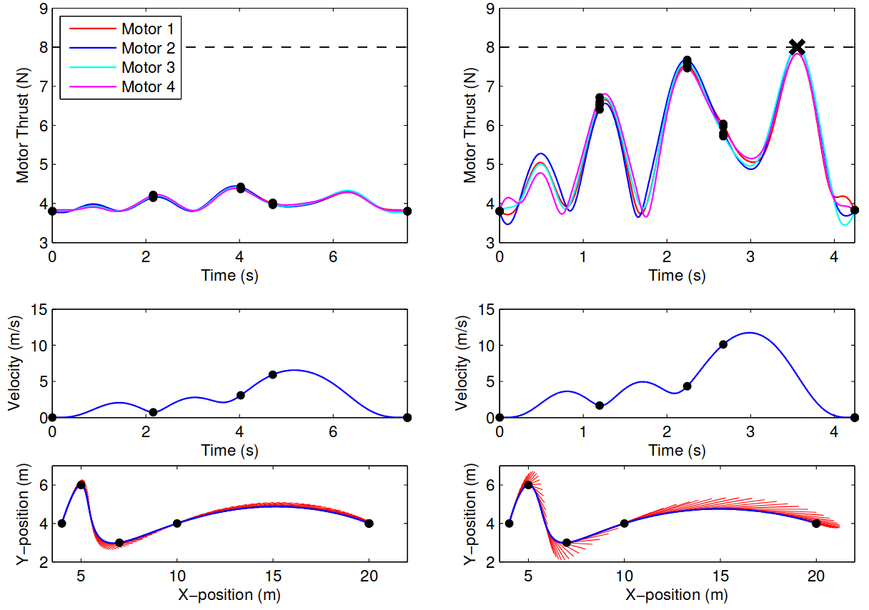
Planning with Obstacles (Mellinger and Kumar 2011)

• At intermediate points, add additional constraints (remains QP)

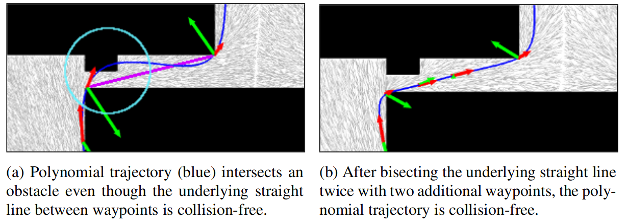
Planning with Obstacles (Richter, Bry, and Roy 2013)

• Use sampling-based geometric planning (RRT) + Optimization
• If there is a collision, add another waypoint

Planning with Obstacles (Richter, Bry, and Roy 2013)

• Or use RRT, with splines in the extent step

Planning with Obstacles (Liu et al. 2018)

• Search-based approach that uses differentially-flatness for edges on A*

YouTube

Double Integrator Assumption

• For many applications double integrator dynamics (and \(\psi=0\)) are used for planning

\[ \begin{align} \mathbf{x}&= [\mathbf{p}, \mathbf{v}]^\top & \mathbf{u}&= [\mathbf{a}]^\top\\ \dot{\mathbf{x}} &= f(\mathbf{x}, \mathbf{u}) = [\mathbf{v}, \mathbf{a}] \end{align} \]

From differential flatness (using \(\dddot{\mathbf{p}} = \mathbf{0}, \dot{\psi}=0\)):

• \(\mathbf{R}, f\) can be recovered from \(\mathbf{a}\)
• \(\boldsymbol{\omega}=\mathbf{0}, \dot{\boldsymbol{\omega}} = \mathbf{0}\)

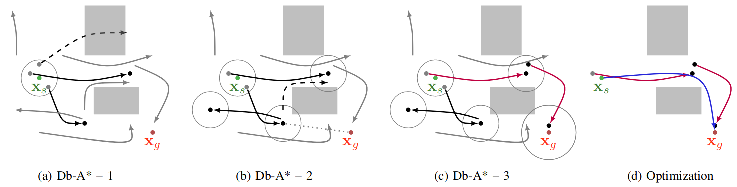
Hybrid Method: db-A* (Ortiz-Haro et al. 2024)

• Differential flatness is incomplete (not all possible motions can be captured), and potentially suboptimal (optimality in the flat space, does not imply optimality in the full space)

• iDb-A*: connect short motion primitives (generated by optimization on the full dynamics) and allow small “jumps”; repair with optimization

Hybrid Method: db-A* (Ortiz-Haro et al. 2024)

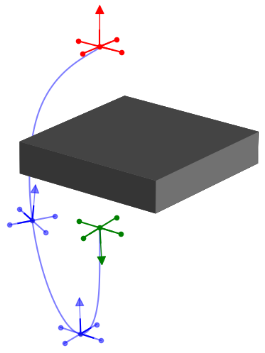
Recovery from up-side down (with low thrust-to-weight ratio).

Planning for Multi-Robot Teams (Hönig et al. 2018)

1. Use discrete search for initial multi-robot path
2. Assign safe corridors, spline optimization within the corridor

YouTube

Planning for Multi-Robot Teams (Moldagalieva et al. 2024)

1. Extend db-A* to the multi-robot world

YouTube

NMPC and/or Motion Planning

• Nonlinear Model Predictive Control (NMPC) solves the kinodynamic motion planning problem for a fixed (typically short) horizon
• Motion planning has \(T\) as decision variable

Planning in the Crazyflie Firmware

• Trajectories are represented as 8th order polynomial splines

• On-board planner uses closed-form solution for goTo (given start position, velocity, acceleration, compute a single spline segment that ends at a desired position with all derivates zero)

• Takeoff/Landing uses the exact same spline planner

• Code (Low-Level)

• Code (High-Level)

Optimization on the Crazyflie

• One can solve (small) QPs on-board using
  • OSQP
  • tinyMPC

Both have tools that generate specific C-Code from a high-level (Python) specification.

Optimization in Rust

• Optimization Engine
  • nonconvex, constrained optimization
  • For “embedded” applications (meaning RPI etc.)
• argmin
  • only unconstrained problems
• Clarabel
  • Convex optimization, state-of-the-art solver
  • Not for embedded
  • Might be supported in cvxpygen in the future
• tinyMPC.rs
  • Uses no_std, but nalgebra; not ported to uC

Task

Generative and validate an aggressive trajectory, exploiting the differential flatness. For planning, use 8th-order polynomial splines that are smooth up to and including snap. For validation, propagate the actions (force, torque) generated by differential flatness using your simulator and compare the result with the expected values and your controller.

Notes

• Only simulation, no flight tests
• Temporal scaling not needed
• Recommended to use Python (cvxpy) for the optimization, not Rust

Timeline

• Feb 7: discussion
• Feb 14: discussion/simulation presentation, oral exam, grading

Learned Today

• Motion Planning for multirotors
  • Differential flatness: \(\mathbf{p}, \psi\) + derivatives map to \(\mathbf{x}, \mathbf{u}\)
  • Planning using polynomial splines
  • Advanced planning methods (hybrid, multi-robot)
• Assignment 4

Questions

References / Suggested Reading